Detection of irrigation inhomogeneities in an olive grove using the NDRE vegetation index obtained from UAV images

January 19, 2019

⊕
https://doi.org/10.1080/22797254.2019.1572459

We have developed a simple photogrammetric method to identify heterogeneous areas of irrigated olive groves and vineyard crops using a commercial multispectral camera mounted on an unmanned aerial vehicle (UAV). By comparing NDVI, GNDVI, SAVI, and NDRE vegetation indices, we find that the latter shows irrigation irregularities in an olive grove not discernible with the other indices. This may render the NDRE as particularly useful to identify growth inhomogeneities in crops. Given the fact that few satellite detectors are sensible in the red-edge (RE) band and none with the spatial resolution offered by UAVs, this finding has the potential of turning UAVs into a local farmer’s favourite aid tool.

J. Jorge¹, M. VallbéDepartment of Mining, Industrial and ICT Engineering, Manresa School of Engineering, Universitat Politècnica de Catalunya, Manresa, Spain. marc.vallbe@upc.edu , and J. A. SolerZCOPTERS, S.L, Viladecans, Spain

European Journal of Remote Sensing, 2019, Vol. 52, No. 1, 169–177

Keywords: remote sensing, unmanned aerial vehicle (UAV), precision agriculture, multispectral, red edge, vegetation indices, crops

Introduction

Remote sensing uses of UAV

Overhead remote sensing data provide complementary input to field inspection and allow for better land surface modelling. In agriculture, most remote-sensing indicators come from photometric indices built using broad-band passbands known as vegetation indices (VI). Although a conventional photographic RGB camera can be used to generate topographic surveys and orthoimages, it takes a multispectral camera covering the visible and IR bands to make differentiating analyses of the landcover using standardised methods of image processing with a prior knowledge of the corresponding spectral signatures. Hence, the combination of modern high spatial resolution and multispectral band sensors offers the possibility to study crops for precision agriculture.Guo, Kujirai, & Watanabe, 2012; Primicerio et al., 2012

Orbiting satellites and manned aircraft have been the traditional platforms to obtain surface photometry. However, they present some limitations in terms of spatial, temporal, and/or spectral resolutions.Nebiker, Annen, Scherrer, & Oesch, 2008 Nowadays, these shortcomings can be overcome using low-cost and flexible unmanned platforms as a good alternative to traditional remote sensing platforms for different applications.Colomina & Molina, 2014; Muchiri & Kimathi, 2016; Nex & Remondino, 2014; Pádua et al., 2017; Pajares, 2015 For instance, Matese et al. (2015) concluded that rotor-based UAVs proved to be the most cost-effective solution for monitoring small fields (<5 ha). They also recommended using fixed-wing small UAVs for fields of up to 1 km² with a ground sample distance (GSD) of up to 5 cm pixel⁻¹, and for fields of up to 4 km² area with a GSD greater than 10 cm pixel⁻¹. Table 1 summarises typical spatial resolutions and fields of view for different platforms. It hints that the spatial resolution gap between 1 and 20 cm can be filled by miniature UAVs.

⊕Table 1. Comparison of UAV with other manned airborne and satellite platforms adapted from Candiago, Remondino, De Giglio, Dubbini, and Gatelli (2015)

	Spatial Resolution	Field of View	Cost for Data Acquisition
Satellite	2–15 m	10–50 km	Very high, for high-res imagery
Aircraft (piloted)	0.2–2 m	2–5 km	High
Miniature UAV	1–20 cm	50–500 m	Very low
Ground-based	<1 cm	<2 m	Low

UAV platforms (fixed-wing and rotor-based) can be coupled with a multitude of sensor options for remote sensing including (1) visual RGB camera (applications in: photogrammetry, aerial mapping, DSM, surveying); (2) multispectral camera (precision agriculture, water quality, vegetation indices, environmental studies); (3) LiDAR (DEM, DSM, 3D surface modelling, object identification, utilities management); (4) thermal IR camera (search and rescue, power line inspection, security, precision agriculture, cell tower inspection, emergency response); (5) hyperspectral camera (environmental monitoring, pipeline inspection, mining and mineral exploration, remote sensing and analysis).

Hence, all information obtained from UAV surveys helps farmers with small fields in decision-making processes, improving agricultural production, and optimising the resource utilisation. With regular flights, producers can make reliable decisions, thereby saving time and money versus using commercial satellite data. For example, UAVs could be used to study the reaction of some crops to new pesticides, as the high-definition data can be easily and quickly examined in a quantitative way. This process can reliably describe the ground situation and overcome the costs of ground inspections.Nebiker et al., 2008

Related works

Usha and Singh (2013) concluded in a review of potential applications of remote sensing (RS) in horticulture that RS is advancing quickly and showed potential for applications in crop biomass detection, soil properties, soil moisture and nutrient content, green fruit counts, crop yield estimation, damage by biotic and a biotic stress, etc. Mathews and Jensen (2013) estimated the canopy leaf area index (LAI) of a vineyard with a digital camera mounted on a micro-UAV; Matese et al. (2013) mapped the wine vigour of a vineyard and extracted the NDVI index from a high-resolution multispectral camera mounted on an eight-rotor platform; Agüera, Carvajal, and Pérez (2011) measured sunflower nitrogen status with a microdrone and compared those measurements with data collected from a ground-based platform. More complex analyses have been performed using hyperspectral sensors, with an increasing number of spectral bands observed, allowing the estimation of biomass and nitrogen content.Honkavaara et al., 2012; Pölönen, Saari, Kaivosoja, Honkavaara, & Pesonen, 2013 . Zarco-Tejada, González-Dugo, and Berni et al. (2012) focused on the calculation of fluorescence, temperature, and narrow band indices and applied these observations to the water stress detection; they also used data from a hyperspectral sensor to calculate relationships between photosynthesis and chlorophyll fluorescence.Zarco-Tejada, Catalina, González, & Martín, 2013 Lukas et al. (2016) compared the basic growth parameters obtained from a fixed-wing UAV equipped with a NIR camera versus data from Landsat-8. Both platforms showed a high correlation with ground measurements of biomass and nitrogen content but the satellite data had coarser resolution.

Vegetation indices from remote sensing imagery

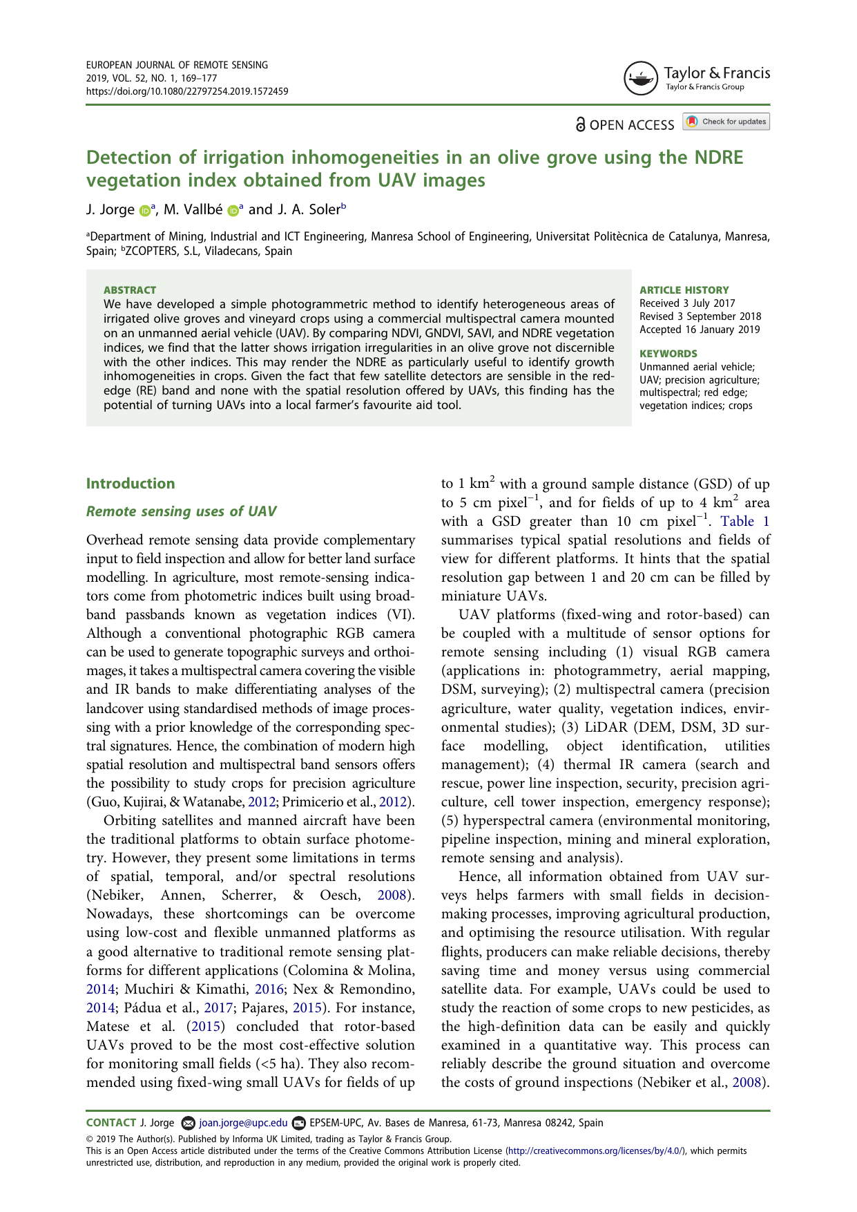
Researchers exploit the fact that vegetation reflectance changes significantly in different passbands to obtain underlying information. As Figure 1 shows, vegetation reflectance is low in both the blue and red regions of the visible spectrum, it peaks locally in the green region, and it is highest in the near infrared (NIR) range. VIs obtained by algebraically combining these bands allow researchers to enhance different spectral signatures for different vegetation properties concerning size, vigour, shape, and colour of leaves.Salamí, Barrado, and Pastor, 2014) Many such VIs have been triedsee review by Xue & Su, 2017 but the most widely used are NDVI, GNDVI, and SAVI.

Figure 1. Spectral reflectance curve for different land covers, with spectral band intervals overplotted.

The normalised difference vegetation index (NDVI), calculated from the reflectance in the NIR and red bands, has been the reference to discuss the state of vegetation since Rouse, Haas., Schell, and Deering (1973). Many studies using it have been published and, for instance, correlations have been found with biomassBendig et al., 2015 , and canopy structure, LAICandiago et al. 2015 .

The green normalised difference vegetation index (GNDVI) has the same form as the NDVI where the red band is substituted by the green band.Gitelson, Kaufman, & Merzlyak, 1996 Hunt, Hively, Daugtry, and McCarty (2008) have shown that it tracks the ratio of photosynthetically absorbed radiation and is correlated with biomass and LAI. This makes the GNDVI more sensitive to chlorophyll content than NDVI.Candiago et al. 2015

Following the lead of Huete (1988) and others, we calculate the soil-adjusted vegetation index (SAVI) to eliminate the effect of soil in areas with poor vegetative cover and where the soil surface is exposed.

Red edge advantage

Despite its many advantages, the NDVI is not always the most accurate index to detect anomalies in crops, particularly if detailed data between the red and NIR bands are available. As shown in Figure 1, there is an abrupt change between the red and NIR reflectance of vegetation, in what is known as the red edge band (RE). This zone marks the limit between absorption by chlorophyll in the red band, and scattering due to leaf internal structure in the NIR band. Being a transition region, the red edge position is very sensitive to changes in the vegetation properties, which can easily be exploited by researchers. For instance, the RE has been used to estimate the chlorophyll content not only of leavesFilella & Peñuelas, 1994; Pinar & Curran, 1996 but also on the surface of waters of a reservoirSchalles, Gitelson, Yacobi, & Kroenke, 1998 . These works led to the formulation of a new vegetation index related to the red edge reflectance, the normalised difference red edge (NDRE), which has been proved more advantageous than the NDVI to optimise harvest times based on transitions of photosynthesis activity.Maccioni, Agati, & Mazzinghi, 2001 Table 2 shows the formula of the four vegetation indices compared in our work.

Index	Computation
NDVI (normalised difference vegetation index)	$$NDVI = \frac{\rho_{NIR} - \rho_{R}}{\rho_{NIR} + \rho_{R}}$$
GNDVI (green normalised difference vegetation index)	$$GNDVI = \frac{\rho_{NIR} - \rho_{G}}{\rho_{NIR} + \rho_{G}}$$
SAVI (soil adjusted vegetation index)	$$SAVI = \left( \frac{\rho_{NIR} - \rho_{R}}{\rho_{NIR} + \rho_{R} + L} \right)\left( {1 + L} \right)$$
NDRE (normalised difference red-edge)	$$NDRE = \frac{\rho_{NIR} - \rho_{RE}}{\rho_{NIR} + \rho_{RE}}$$

⊕Table 2. The computed vegetation indices. ρ_G, ρ_R, ρ_RE, and ρ_NIR represent the reflectance in the green, red, red edge, and near infrared band, respectively; L is a constant empirical value related to the vegetation density on the ground (see for example a review by Xue & Su, 2017).

Unfortunately, few remote-sensing satellites carry sensors capable of detecting radiation in the red-NIR transition zone, or RE band. As of today, these include WorldView-3 (not the WorldView-4) with a multi-band spatial resolution of 1.4 m; RapidEye, with 5 m for ground sampling distance; Sentinel-2 satellite, with a spatial resolution of 20 m. Luckily, most commercial multispectral cameras that are installed in UAVs detect RE radiation, and this opens a niche for these smaller platforms. For instance, there are 400 7-cm spatial resolution pixels for each 1.4-m resolution pixel of the red-edge band of WorldView-3. This makes a significant difference for precision agriculture since it can unmask relevant details.

This paper reports a study done on 13 ha of farm land using a multiband (visible and NIR) camera and a photometer onboard a UAV. Several different vegetation indices have been applied to an area where vegetation is represented by fields of olive groves and vineyards, with the aim of discerning how the red-edge band might improve our agricultural knowledge on small fields. Hence, we compare the vegetation indices, notably the NDRE index against the other usual VI.

Materials and methods

Overview

This study evaluates the results and potential of green versus red versus red edge versus NIR images to obtain maps of vegetation indices to detect inhomogeneities in irrigated crops. In particular, our work comprises the following:

The photogrammetric planning and processing of multispectral datasets acquired with a commercial camera mounted on a UAV platform.
The creation of high-resolution orthophotos from multispectral images over two different cultivation areas (vineyard, olive grove).
The generation and evaluation of different VI maps.
Statistical analysis of the VIs crossing their values for two types of crops.

These steps were performed with a critical approach to understanding the easiest and most efficient way to deliver geo-referenced information at small spatial scales useful for precision farming. Our final aim was to discriminate vegetation of the same crop with different response to the aforementioned vegetation indices without any ground radiometric measure. Careful descriptions of the agricultural characteristics provided by local farmers who manage the different crops sites were used to validate the findings.

Study area

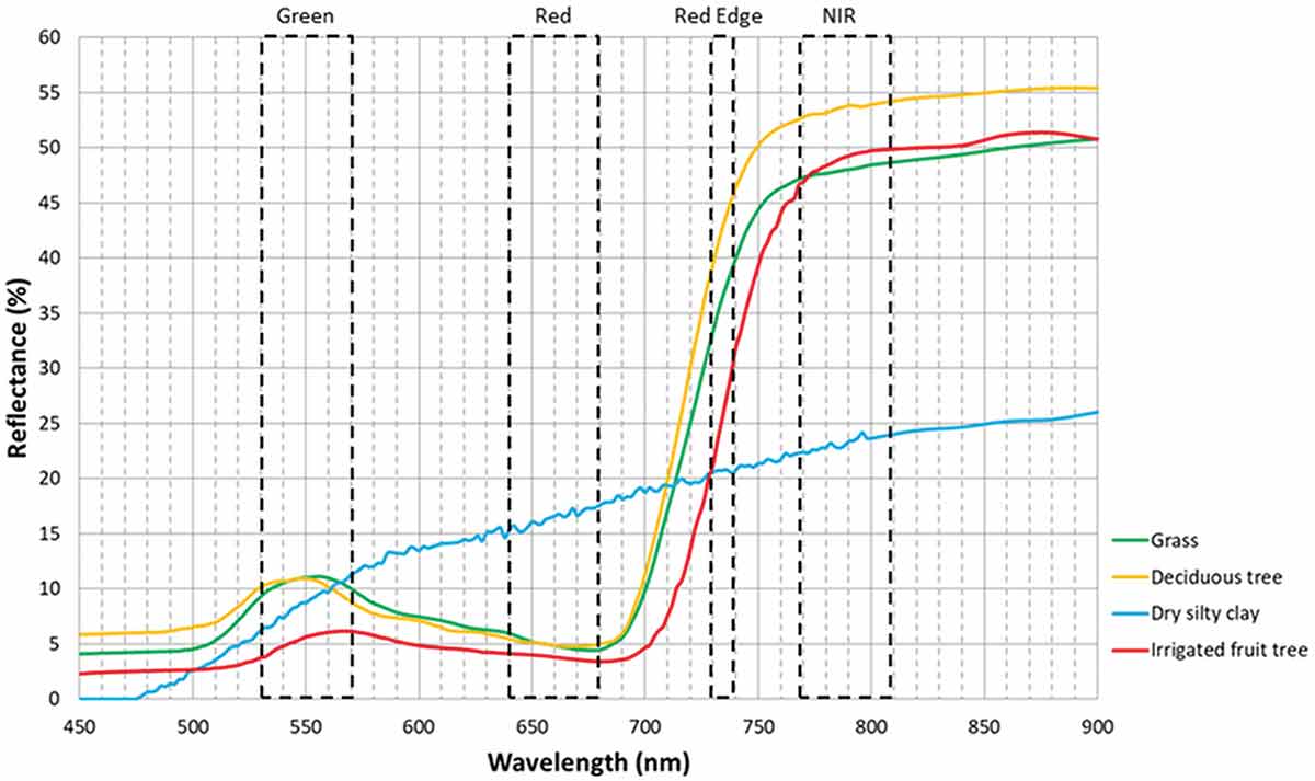
The study area corresponds to a rural property located near Manresa (Barcelona), called “Celler el Molí”http://www.cellerelmoli.com , coordinates 41º44ʹ14.36″N, 1º46ʹ47.94″E (UTM 46213331.284, 398545.852), datum WGS84, with altitudes between 298 and 344 m above sea level with no or just a slight slope. The area enjoys a Mediterranean continental climate with a notable thermal oscillation. The lands are mainly loamy soils.

Figure 2. Location of the study site, 60 km west of Barcelona (red dot on the maps on the left-hand side). The right figure shows an aerial view of the site.

The study site has an area of approximately 13 ha and includes the housing of the farmers and the winery. In this location, there are invariant places, such as buildings, parking lots, and roads, whose coordinates could be registered to assess the quality of the orthomosaicked image (Figure 2). There are different plots with two typical Mediterranean crops. The farm land is divided into olive groves and vineyards. The dominant crop is organic vineyard, with four grape varieties: Cabernet, Macabeu (native from Catalonia), Merlot, and Picapoll (native from Catalonia). Some vineyard plots are drip irrigated while other plots are not irrigated (see Table 3 and Figure 6), even if they are of the same grape variety. The wine that is produced with these grapes has the denomination of origin Pla de Bages.http://www.dopladebages.com/ The dominant olive variety is Arbequina (native from Catalonia). The crop is a super high-density plantation, with a linear structure with virtually no distance between trees and a narrow corridor between rows, and the land covered by legumes to avoid erosion and also to enrich the soil, thus favouring the biological cycles (legumes fix nitrogen which will be exploited by olive trees). The olive grove is subject to a drip irrigation system by micro irrigation pipes.

Data collection and preprocessing

The employed UAV platform was a quadcopter Phantom 4 Pro, designed and produced by DJI and provided with a commercial multispectral camera. For this work, a Parrot Sequoia 4.0 camera was used. This camera is a powerful multispectral sensor in a pocket-sized package, has a weight of 90 g, it spans 75 mm × 59 mm × 33 mm, integrates a GPS/light sensor, and the camera’s sensor acquires images 5,472 × 3,648 pixels in four narrowband imagers. The spectral ranges of the four bands are Green (530–570 nm), Red (640–680 nm), Red Edge (730–740 nm), and NIR (770–810 nm). The camera is complemented by a sunshine sensor and a reflectance calibration plate for each of the multispectral bands, so that the data provided by the set are essentially reflectance values instead of just grey level.

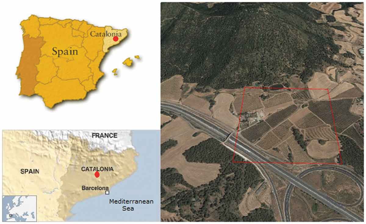
To cover the entire study area, 276 images were captured for each of the four spectral bands in a first flight (GSD of 6.8 cm pixel⁻¹). An RGB camera mounted in the UAV in a second flight allowed us to capture 239 images in the visible spectrum (24,144 × 23,700 pixels, and 0.017 m of GSD) with some overlap, which allowed us to elaborate a mosaic of orthorectified images resulting from the preprocessing operations (involving homographic corrections and stitching) upon the acquired images. The photogrammetric processing was performed using proprietary Pix4D software (Pix4D SA, Lausanne, Switzerland). The process follows three steps: (1) aerial triangulation; (2) digital surface model generation, and (3) orthomosaicking. The resulting orthomosaicked images have high resolutions and are accurate throughout consecutive images. Thus, they guarantee optimal performance of the subsequent classification analysis. After that, the data from the two flights were joined to manage, transform, and export the images (four different images, one for each channel) to a TIFF format. 239 images were calibrated and geolocated using 27,657 matches per calibrated image. In this way, the quality of the image content was evaluated to test its influence on the outcomes of the photogrammetric processing and vegetation indices.

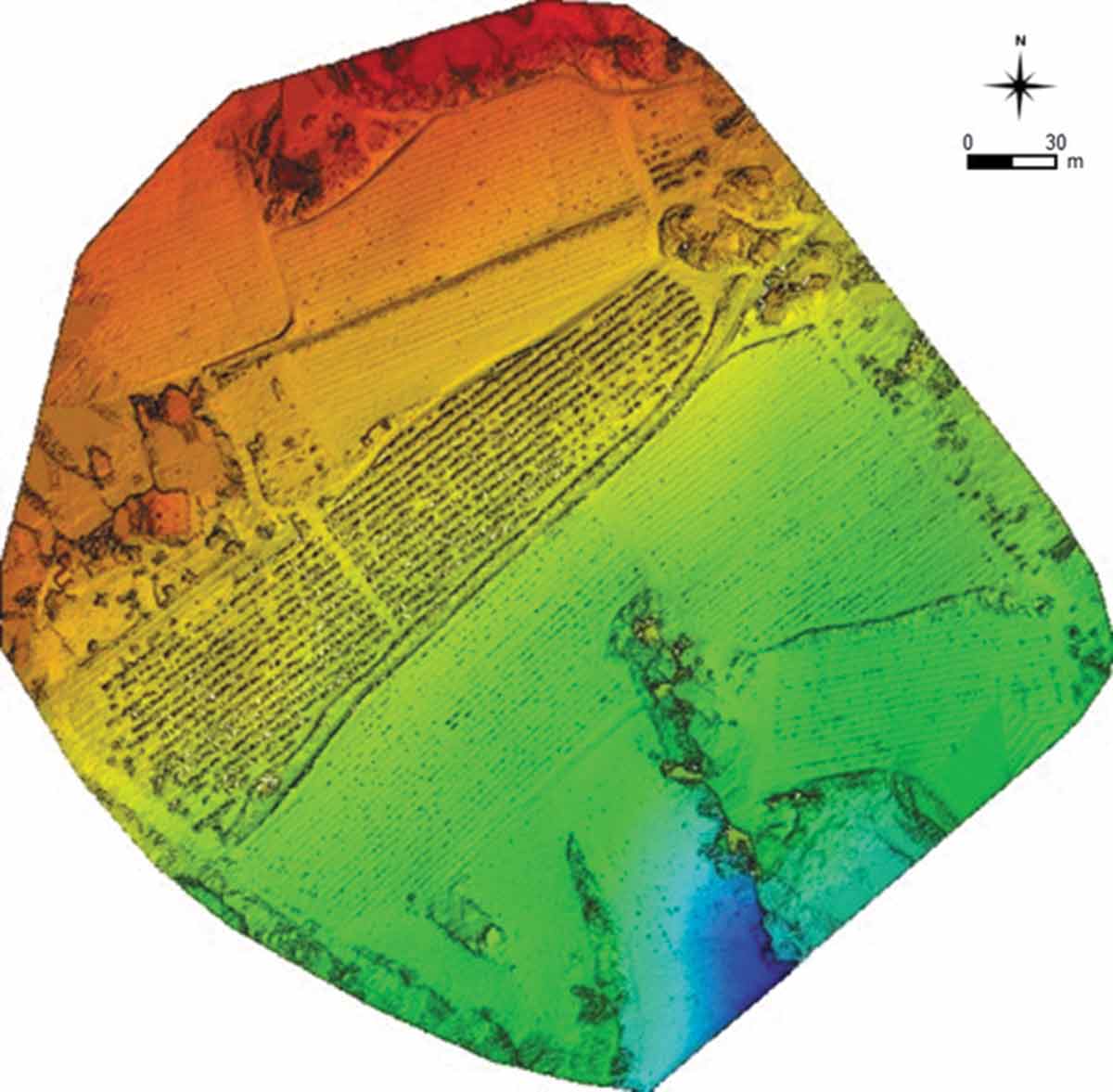
Figure 3 shows the orthorectified image mosaic without a georeferenced legend and with the flight line and point cloud superimposed. Figure 4 shows the sparse digital surface model (DSM) before densification obtained in the previous process.

Figure 3. Preprocessing steps with Pix4D software for 239 RGB images: orthorectified image mosaic, with the flight line and point cloud superimposed.

Figure 4. Sparse digital surface model (DSM) before densification obtained in the preprocessing process. Redder colours correspond to greater heights.

It should be indicated that in absence of ground measurements with spectro-radiometers, the computations of raw indices might be based on digital numbers (DN), or grey levels. Although the raw indices give a good description of the vegetation conditions, it is possible that the traditional scale ranges of the vegetation indices used are affected somewhat.

Image classification

Before building the vegetation indices, an unsupervised classification of the images was done in order to have a proto image of homogeneity in the crops. Figure 5 shows the resulting classification map after having visited the farm and verified the ground truth personally in situ, reducing the number of classes by merging them and deleting noisy pixels. Only four surface classes are differentiated: the blue colour is associated to bare soil with a small roughness (roads and vines just planted); the shade of lighter green corresponds to the legumes that are between the rows of olive trees; the darkest green corresponds to the rougher bare soil between the vines; and the orange colour corresponds to the productive olive trees and the vines.

Figure 5. Unsupervised classification of the farm into four classes.

Vegetation indices results

The vegetation indices used to create vigour maps and to verify uniform growth of the crops were calculated using the raster calculator tool of QGIS, which was also used to build the maps. The VI calculation was done by applying the standard formulations (Table 2) within the limited geographical extent where the four spectral bands (G, R, RE, and NIR) were recorded. The reflectance images were obtained from their respective band indices which were procured from the preprocessing (orthorectification) performed with the Pix4D software, as mentioned before. Each resulting image has a spatial resolution of 0.06839 m and shows pixels with reflectance value and other pixels with no data.

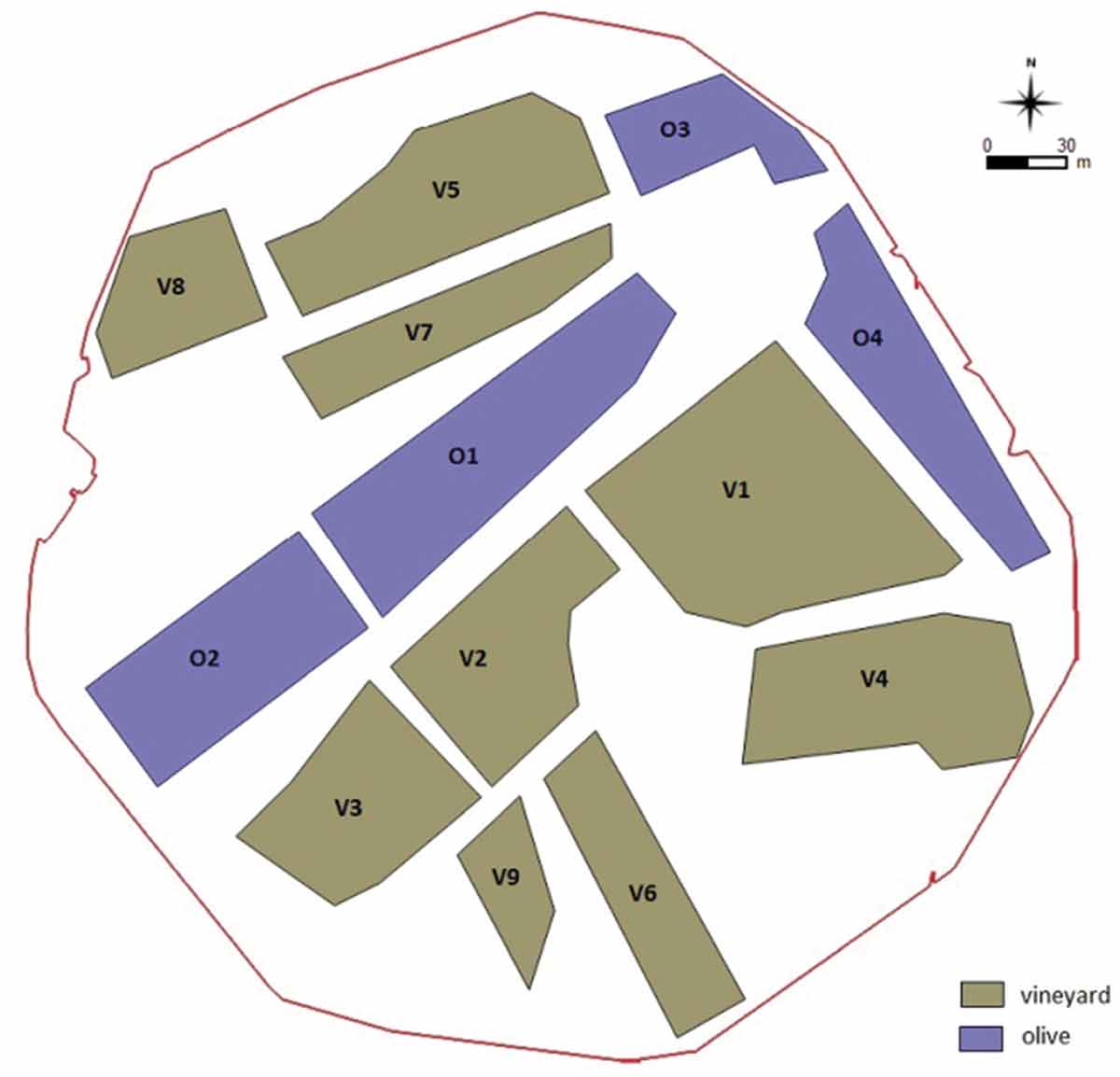
We have differentiated four plots for olive crops (always Arbequina cultivar) and nine for vineyards, which have been used to mask the vegetation indices and to make statistics based on the data for each of them. Figure 6 shows the masks of olive and vine crops that have been applied on maps of vegetation indices. Tables 3 and 4 summarise the extension of each of the masks: 1.71 ha of olive trees and 3.72 ha of vineyard (C: Cavernet, Me: Merlot, Ma: Macabeu, P: Picapoll, R: irrigation, S: no irrigation). For each crop, we have divided the study in different plots identified with a correlative number.

⊕Table 3. Extension (in ha) of the different masks built for the olive grove (O: Arbequina; R: irrigation; S: no irrigation).

Olive
Plot	O1	O2	O3	O4	Total
ha	0.62	0.47	0.22	0.40	1.71

Figure 6. Masks of olive and vines crops applied on maps of vegetation indices.

Vineyard
Plot	V1	C1	V1	V2	V3	V4	V5	V6	V7	V7	V8	V9	Total
	C	Me1	Me2	C	C	Me	C	P	Ma1	Ma2	C	Ma
	R	R	R	S	S	S	R	S	R	R	S	S
ha	0.25	0.23	0.29	0.45	0.40	0.52	0.54	0.33	0.12	0.21	0.26	0.14	3.72

⊕Table 4. Extension (in ha) of the different masks built for the vinyard (C: Cabernet; Me: Merlot; Ma: Macabeu; P: Picapoll; R: irrigation; S: no irrigation).

The olive crops

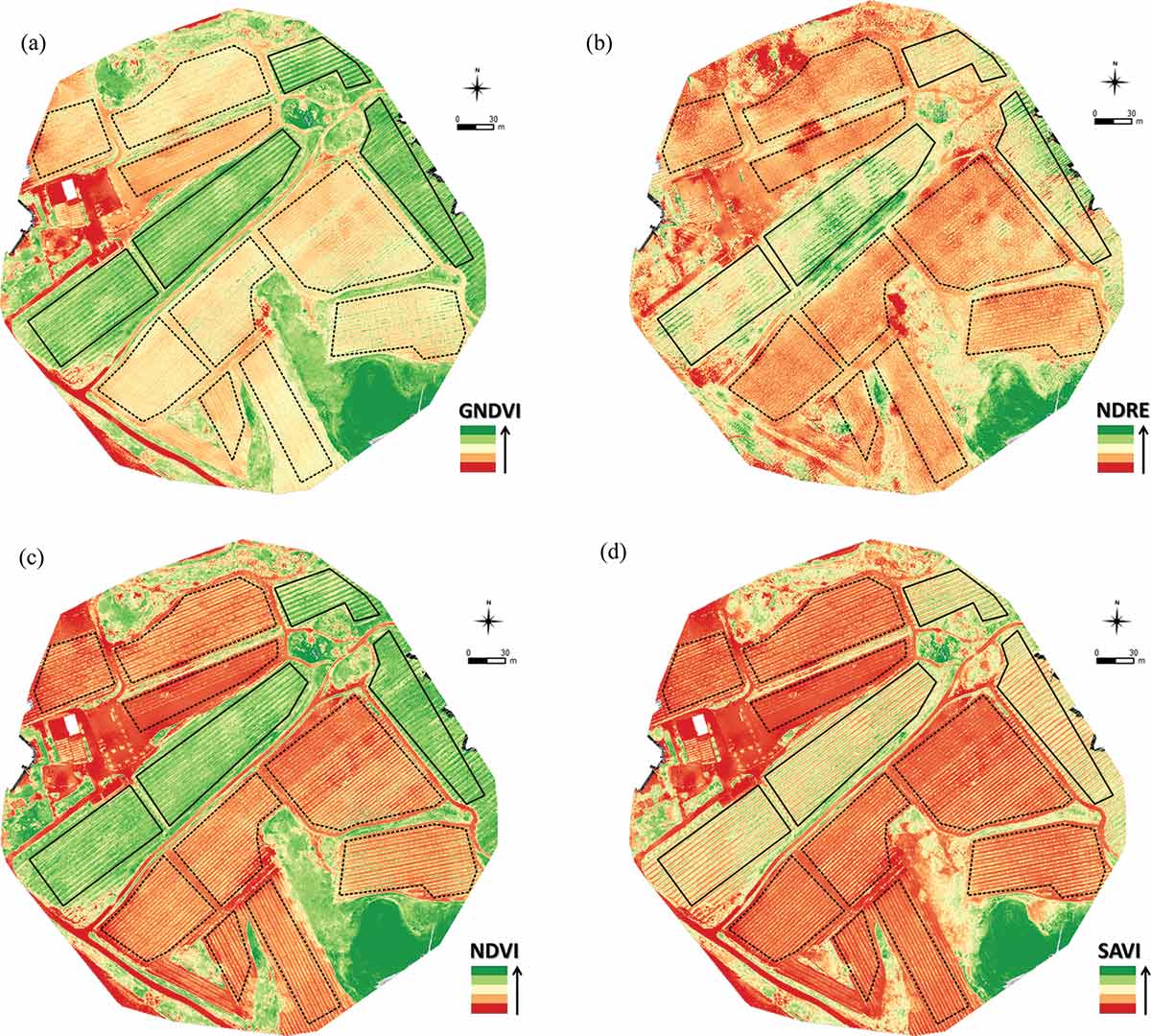
The NDVI, GNDVI, SAVI (L = 0.2, 0.5, 0.9), and NDRE indices maps for olive crops were extracted from the processed orthoimage. After comparing the minimum, maximum, mean, and standard deviation values of the VIs for the selected plots, we discarded to continue working with the values of SAVI (L = 0.2) and SAVI (L = 0.9), and concentrated only on the SAVI (L = 0.5) because all of them showed similar correlations to the rest of VIs. In the literature on remote sensing, vegetation indices, and agriculture, it is customary to use this index only with the soil parameter L = 0.5. Figure 7 shows the map values of the estimated VIs for the olive areas. The different values of the legend of each of the maps can be observed.

Figure 7. Images of the various vegetation indices for the olive (continuous line) and vineyard plots (dashed line): (a) GNDVI, (b) NDRE, (c) NDVI, (d) SAVI (L = 0.5).

After differentiating the plots of olive trees and applying their mask to the maps obtained for each of the VI, we proceeded to analyse the linear correlation that may exist between the different VI considering the whole set of pixels, regardless of the class of cover they represented. Table 5 shows the R-squared values obtained when correlating the different VIs with the NDVI and with the NDRE for each plot of olive grove.

⊕Table 5. R-squared values obtained when correlating the different VIs with the NDVI and with the NDRE for the plots of olive grove.

	O1	O2	O3	O4	Total
R² correlation with NDVI (olive)
GNDVI	0.79	0.86	0.93	0.71	0.83
NDRE	0.41	0.43	0.53	0.27	0.37
SAVI (L = 0.5)	0.44	0.36	0.51	0.36	0.37
R² correlation with NDRE (olive)
GNDVI	0.41	0.49	0.60	0.42	0.43
NDVI	0.41	0.43	0.53	0.27	0.37
SAVI (L = 0.5)	0.29	0.06	0.18	0.14	0.18

The vineyard crops

For the vineyard crops we have proceeded in the same way as for olive crops. The NDVI, GNDVI, SAVI (L = 0.2, 0.5, 0.9), and NDRE indices maps for vine crops were extracted from the processed orthoimage. After comparing the minimum, maximum, mean, and standard deviation values of the VIs for the selected plots, we decided to work with SAVI (L = 0.5) and not with SAVI (L = 0.2) and SAVI (L = 0.9) for the same reasons mentioned before. Figure 7 shows the map values of the estimated VIs for the vine crops.

After differentiating the plots of vineyard and applying their mask to the maps obtained for each of the VI, we proceeded to analyse the linear correlations that may exist between the different VI considering the whole set of pixels, regardless of the class of cover they represented. Table 6 shows the R-squared values obtained when correlating the different VI with the NDVI and with the NDRE for each plot of vineyard.

	V1_C_R	V5_C_R	V2_C_S	V3_C_S	V8_C_S	V6_P_S	Total
R² correlation with NDVI (vineyard)
GNDVI	0.89	0.83	0.92	0.85	0.72	0.61	0.87
NDRE	0.47	0.28	0.32	0.18	0.12	0.23	0.40
SAVI (L = 0.5)	0.98	0.94	0.96	0.95	0.97	0.97	0.96
R² correlation with NDRE (vineyard)
GNDVI	0.50	0.28	0.40	0.30	0.09	0.14	0.41
NDRE	0.47	0.28	0.32	0.18	0.12	0.23	0.40
SAVI (L = 0.5)	0.43	0.19	0.29	0.03	0.08	0.14	0.33

⊕Table 6. R-squared values obtained when correlating the different VIs with the NDVI and with the NDRE for the plots with vineyard crops (C: Cabernet; Me: Merlot; Ma: Macabeu; P: Picapoll; R: irrigation; S: no irrigation).

Discussion

The results shown in the previous section reveal the convenience to work with several vegetation indices to detect irregularities in the crops. In the case of olives, the traditional NDVI shows a fairly elongated homogeneity compared to the other indices we have applied. NDRE is especially useful to detect small areas with different textures within the cultivated plots. In these areas, the farmer may wish to collect information in situ.

In our case, we observe an inhomogeneity in the centre of the plot O1 which is most conspicuous in the NDRE. On site inspection confirmed that this inhomogeneity is due to less vigorous vegetation. At first, this seemed odd since every tree received the same amount of water and at the same time (the same overall treatment, in fact), so these variables do not play a role in the irregularity detected. However, during the inspection, the farmers noted that there used to be a stream running through the centre of the plot, which they covered with new soil to flatten the land just before planting the olive trees a few years ago. This explains why in this area the vegetation is less vigorous, given that there is likely less water retained in the first shallow inches of subsoil (where the roots of the young olive trees have access) due to percolation through the new added soil – which is less compacted and hence more porous than consolidated soil.

The differences between NDVI, GNDVI, and NDRE should not be surprising when we take into account the spectral signature of the vegetation shown in Figure 1. Despite the difference in absolute values, there is an excellent correspondence between the NDVI and GNDVI indices (R² = 0.83 for olive; R² = 0.87 for vineyard). In the case of NDRE, the correlation is quite poor with NDVI (R² = 0.37 for olive; R² = 0.40 vineyard), similar with GNDVI and worse with SAVI. This is likely due to the bigger dispersion of reflectance values in the RE than in the R band when water and nitrogen content change.Mutanga & Skidmore, 2007 The correlation data between the different VIs are exceptionally high for NDVI and SAVI in the case of vines (R² = 0.96) and low for olive (R² = 0.37). This difference is due to the difference in percentage of vegetation cover (being the vines very young and the bare soil dominates the image). The worst correlation is obtained between NDRE and SAVI for olive crop (R² = 0.17); it may be due to the sensitivity of the SAVI to a variety of soil textures not covered by vegetation.

Conclusions

In this paper, we report a study involving the use of UAVs in precision agriculture based on the comparison of vegetation indices calculated from multispectral images (G, R, RE, NIR) of high spatial resolution (6.8 cm pixel⁻¹). These high resolution data allow for a fairly detailed characterisation of the biophysical variables of the crops. After comparing vegetation index maps incorporating the red edge band, the use of NDRE instead of the traditional NDVI can be recommended to identify possible heterogeneities in the vegetation cover, even when the vegetation does not fully cover the ground and patches of bare soil with varying degrees of roughness are the norm. To our knowledge, this is the first time that the NDRE has been used to trace irrigation irregularities in olive crops. This has important consequences for local farmers who now have affordable UAVs to perform live assessments of their crops. It would be very useful to precision agriculture if more RE detectors were put onboard satellites.

Acknowledgments

The authors would like to thank the kind attention of Mr. Josep Mª Claret (Celler el Molí), responsible for the agricultural activity, for providing us with access to the farm, the corresponding agronomical reference data and for his agronomical advice on the interpretation of the results. We also appreciate the collaboration of Mr. J. Quesada (MAPDRONE S.L.).

Disclosure statement

No potential conflict of interest was reported by the authors.

References

Agüera, F., Carvajal, F., & Pérez, M. (2011, September 14–16). Measuring sunflower nitrogen status from an unmanned aerial vehicle-based system and an on the ground device. In Proceedings of the Conference on Unmanned Aerial Vehicle in Geomatics (Vol. 38 (1/C22)). Zurich, Switzerland.

Bendig, J., Yu, K., Aasen, H., Bolten, A., Bennertz, S., Broscheit, J., & Bareth, G. (2015). Combining UAV-based plant height from crop surface models, visible, and near infrared vegetation indices for biomass monitoring in barley. International Journal of Applied Earth Observation and Geoinformation, 39, 79–87. Crossref.

Candiago, S., Remondino, F., De Giglio, M., Dubbini, M., & Gatelli, M. (2015). Evaluating multispectral images and vegetation índices for precisión farming applications fron UAV images. Remote Sensing, 7(4), 4026–4047. Crossref.

Colomina, I., & Molina, P. (2014). Unmanned aerial systems for photogrammetry and remote sensing: A review. ISPRS Journal of Photogrammetry and Remote Sensing, 92, 79–97. Crossref.

Filella, I., & Peñuelas, J. (1994). The red edge position and shape as indicators of plant chlorophyll content, biomass and hydric status. International Journal of Remote Sensing, 15(7), 1459–1470. Crossref.

Gitelson, A.A., Kaufman, Y.J., & Merzlyak, M.N. (1996). Use of a green channel in remote sensing of global vegetation from EOS-MODIS. Remote Sensor Environment, 58(3), 289–298. Crossref.

Guo, T., Kujirai, T., & Watanabe, T. (2012). Mapping crop status from an unmanned aerial vehicle for precision agriculture applications. ISPRS - International Archives of the Photogrammetry, Remote Sensing and Spatial Information Sciences, 39(B1), 485. Melbourne, Australia. Crossref.

Honkavaara, E., Kaivosoja, J., Mäkynen, J., Pellikka, I., Pesonen, L., Saari, H., … Rosnell, T. (2012, August 25–September 1). Hyperspectral reflectance signatures and point clouds for precision agriculture by light weight UAV imaging system. In Proceedings of the XXII ISPRS Congress, (Vol. I-7, pp. 353–358), Melbourne, Australia. Crossref.

Huete, A.R. (1988). A soil adjusted vegetation index (SAVI). Remote Sensing of Environment, 25(3), 295–309. Crossref.

Hunt, J., Hively, W.D., Daugtry, C.S.T., & McCarty, G.W. (2008, November 18–20). Remote sensing of crop leaf area index using unmanned airborne vehicles. In Proceedings of the Pecora 17 Conference, American Society for Photogrammetry and Remote Sensing, Denver, Colorado.

Lukas, V., Novák, J., Neudert, L., Svobodova, I., Rodriguez-Moreno, F., Edrees, M., & Kren, J. (2016, July 12–19). The combination of UAV survey and Landsat imagery for monitoring of crop vigor in precision agriculture. In The International Archives of the Photogrammetry, Remote Sensing and Spatial Information Sciences, Volume XLI-B8, 2016 XXIII ISPRS Congress, Prague, Czech Republic. Crossref.

Maccioni, A., Agati, G., & Mazzinghi, P. (2001). New vegetation indices for remote measurement of chlorophylls based on leaf directional reflectance spectra. Journal of Photochemistry and Photobiology B: Biology, 61(1–2), 52–61. Crossref.

Matese, A., Capraro, F., Primicerio, J., Gualato, G., Gennaro, S.F.D., & Agati, G. (2013). Mapping of vine vigor by UAV and anthocyanin content by a non-destructive fluorescence technique. In: Stafford J.V. (eds) Precision agriculture, 13. Wageningen Academic Publishers, Wageningen.

Matese, A., Toscano, P., Di Gennaro, S.F., Genesio, L., Vaccari, F.P., Primicerio, J., & Gioli, B. (2015). Intercomparison of UAV, aircraft and satellite remote sensing platforms for precision viticulture. Remote Sensing, 7(3), 2971–2990. Crossref.

Mathews, A.J., & Jensen, J.L.R. (2013). Visualizing and quantifying vineyard canopy LAI using an unmanned aerial vehicle (UAV) collected high density structure from motion point cloud. Remote Sensing, 5, 2164–2183. Crossref.

Muchiri, N., & Kimathi, S. (2016). A review of applications and potential applications of UAV. Proceedings of Sustainable Research and Innovation Conference, 0, 280–283, Nairobi, Kenya.

Mutanga, O., & Skidmore, A.K. (2007). Red edge shift and biochemical content in grass canopies. ISPRS Journal of Photogrammetry and Remote Sensing, 62(1), 34–42. Crossref.

Nebiker, S., Annen, A., Scherrer, M., & Oesch, D. (2008). A light-weight multispectral sensor for micro UAV—opportunities for very high resolution airborne remote sensing. The International Archives of the Photogrammetry, Remote Sensing and Spatial Information Sciences, XXXVII(B1), 1193–1200.

Nex, F., & Remondino, F. (2014). UAV for 3D mapping applications: A review. Applied Geomatics, 6, 1–15. Crossref.

Pádua, L., Vanko, J., Hruška, J., Adão, T., Sousa, J.J., Peres, E., & Morais, R. (2017). UAS, sensors, and data processing in agroforestry: A review towards practical applications. International Journal of Remote Sensing, 38(8–10), 2349–2391. Crossref.

Pajares, G. (2015). Overview and current status of remote sensing applications based on unmanned aerial vehicle (UAV). Photogrammetric Engineering & Remote Sensing, 81(4), 281–329. Crossref.

Pinar, A., & Curran, P.J. (1996). Grass chlorophyll and the reflectance red edge. International Journal of Remote Sensing, 17(2), 351–357. Crossref.

Pölönen, I., Saari, H., Kaivosoja, J., Honkavaara, E., & Pesonen, L. (2013). Hyperspectral imaging based biomass and nitrogen content estimations from light-weight UAV. In Proc. SPIE, 8887, Crossref.

Primicerio, J., Di Gennaro, S.F., Fiorillo, E., Genesio, L., Lugato, E., Matese, A., & Vaccari, F.P. (2012). A flexible unmanned aerial vehicle for precision agriculture. Precision Agriculture, 13, 517–523. Crossref.

Rouse, J.W., Haas., R.H., Schell, J.A., & Deering, D.W. (1973, December 10-14). Monitoring vegetation systems in the great plains with ERTS. In Proceedings of the Third ERTS Symposium (pp. 309–317) Washington, DC: NASA. NASA SP-351.

Salamí, E., Barrado, C., & Pastor, E. (2014). UAV flight experiments applied to the remote sensing of vegetated areas. Remote Sensing, 6(11), 11051–11081. Crossref.

Schalles, J.F., Gitelson, A., Yacobi, Y.Z., & Kroenke, A.E. (1998). Chlorophyll estimation using whole seasonal, remotely sensed high spectral-resolution data for an eutrophic lake. Journal of Phycology, 34, 383–390. Crossref.

Usha, K., & Singh, B. (2013). Potential applications of remote sensing in horticulture—A review. Scientia horticulturae, 153, 71–83. Crossref.

Xue, J., & Su, B. (2017). Significant remote sensing vegetation indices: A review of developments and applications. Journal of Sensors, 2017, 17. Article ID 1353691. Crossref.

Zarco-Tejada, P.J., Catalina, A., González, M.R., & Martín, P. (2013). Relationships between net photosynthesis and steady-state chlorophyll fluorescence retrieved from airborne hyperspectral imagery. Remote Sensing of Environment, 136, 247–258. Crossref.

Zarco-Tejada, P.J., González-Dugo, V., & Berni, J.A.J. (2012). Fluorescence, temperature and narrow-band indices acquired from a UAV platform for water stress detection using a micro-hyperspectral imager and a thermal camera. Remote Sensing of Environment, 117, 322–337. Crossref.